Introduction
Flooding is one of the major causes of socioeconomic loss and losses to humans and poses a potential danger in urban areas located downstream of large river basins. Accurate real-time flood forecasts will significantly reduce the potential damage caused by flooding. Many predictive measures have been proposed to mitigate and prevent the effects of floods, and require a large amount of data for forecasting. There are currently two approaches to streamflow forecasting. The first method relies heavily on the use of mathematical models that simulate the hydrodynamic processes of the streamflow. This option is widely used in Vietnam and other countries worldwide as it is based on the original hydrology and hydraulic concepts. However, a drawback of this approach is that it requires a large amount of input data. Moreover, the parameters of the model must be validated and evaluated carefully, but sometimes it is difficult to select suitable parameters for the model.
The second approach is data-driven and is based on the statistical relationship between input and output data for near-future predictions. One of the most prevalent models used in the data-driven method is the artificial neural network (ANN) model, which has been used in flood forecasting since the 1990s. In addition, researchers have applied state-of-the-art algorithms to the ANN model to increase the accuracy of the predicted results. With the breakthrough development of information technology and the field of computer science, the data-driven approach is now an effective alternative to conventional hydrological prediction methods (Kişi, 2011) that are closely related to hydrodynamic models owing to the simplicity of building the models structure and the modest amount of data required. Several studies conducted worldwide and in Vietnam using the ANN model-based approach are summarized below.
Elsafi (2014) proposed an ANN model for flow forecasting at Dongola station on the Nile River, Sudan. The model was constructed using observed flowrate data obtained at upstream hydrological stations to simulate the flowrate at Dongola station. The results indicate that the ANN model is highly reliable for detecting flood disasters in the Nile River basin. Another ANN model was used to predict the flowrate in the Tomebamba River, Ecuador by Veintimilla-Reyes et al. (2016). The input data of the model were rainfall and discharge data measured at the hydrological stations along the river. They concluded that this model produces highly reliable predictive results when forecasting the three-day flowrate, and this result can be used to avoid disaster flooding in Cuenca City, downstream of the river basin. Sung et al. (2017) developed an ANN model based on hourly water level data obtained upstream to predict the water level in the Anyangcheon River basin one to three hours ahead. The study demonstrated that the proposed model performed well when predicting one or two hours in advance, however, the three-hour predicted water level was not accurate. Several other studies in the hydrological field have successfully applied a data-driven approach to predict streamflow (Hidayat et al., 2014; Aichouri et al., 2015; Wang et al., 2017) or water levels (Seo et al., 2015).
Studies on streamflow forecasting in Vietnam with a data-driven approach are limited, and are only available for some river basins. Some of the studies following method are listed below. Truong and Nguyen (2016) predicted the incoming flow of the Hoa Binh reservoir at Ta Bu station using a deep learning model, which is an intense application of the ANN model. The data used in the model were 39 years of dry season observation data from 1964 to 2002, with a measured time step of 10 days. The authors used this data to predict the flowrate 10 days ahead at Ta Bu station. The model generates predictable results with an accuracy of up to 92%, which is higher than that of other methods. Le and Ho (2018) developed a long short-term memory (LSTM) model (an application of the DNN model) to predict the water levels at two gauge stations in Hai Phong city. The Quang Phuc and Cua Cam hydrological stations are located in Hai Phong city where the water level is affected by tidal fluctuations. This model requires hourly precipitation and water level input data to forecast water levels for one to five hours at the two hydrological stations mentioned above. The predicted results of the model indicated good performance; the Nash-Sutcliffe Efficiency (NSE) value reached 92% for both stations when predicting the five-hour water level. In addition, some studies using deep learning model have also been conducted to predict the streamflow characteristics of river basins in Vietnam (Chen et al., 2014; Nguyen, 2015; Nguyen et al., 2015; Le et al., 2018; Le et al., 2019). These studies demonstrate that DNN-based streamflow forecasting models are becoming increasingly prevalent and accurate (LeCun et al., 2015).
In this study, the authors constructed a DNN model for predicting the flowrate of the Red River at Son Tay station, located in the north-western area of Hanoi. The streamflow forecasts at the Son Tay hydrological station plays a vital role in the early flood warning system for downstream areas and predicting flood flows in downstream rivers. This is because Hanoi is located in the downstream area, the economic, cultural, and political center of Vietnam. The LSTM model developed by the authors is a specialized DNN model that resolves problems relating to sequential data. This model only uses the daily average flow data collected at upstream and target-forecasting stations. The output of the model is the expected incoming flowrate at Son Tay station one, two, and three days in advance. The proposed model also does not require terrain or river basin surface-coverage data.
Materials and Methods
Artificial neural network (ANN)
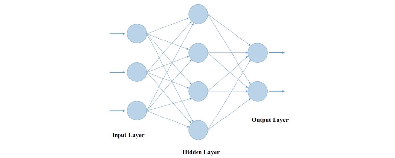
The ANN model is based on the activity of the nervous system and includes a large number of connected neurons for information processing. ANNs can store information and use it to predict unseen data. ANNs typically consist of three components, i.e., input, hidden, and output layers. The relationship between the input and output data is expressed by equation (1) (Govindaraju, 2000a).
 (1)
(1)
where Y is the result of the forecast and X1, X2, ... , Xn are the input data vectors.
These data layers are connected through weight matrices, bias, and several transformation functions. The basic structure of an ANN is presented in Fig. 1.
An ANN model can have one or more hidden layers. The number of hidden layers depends on the shape and size of the input dataset, and the accuracy requirements of the output data. The complexity of an ANN is related to the number of hidden layers and the number of neurons in each hidden layer. In general, there are no specific rules for determining the number of hidden layers or the number of neurons within them. These parameters can be determined based on trial and error evaluation.
According to Govindaraju (2000b), ANN models face issues in understanding watersheds when solving hydrological problems. Another important issue of traditional ANN models is the lack of memory when resolving sequencing data problems. In this study, the authors developed a DNN model, referred to as LSTM, which is an intensive application of the ANN model. The developed model can resolve the predictive problems related to time series.
LSTM neural network
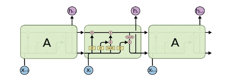
LSTM networks are a specialized type of recurrent neural network (RNN) and were introduced by Hochreiter and Schmidhuber (1997) to resolve the issues related to sequential data. A typical LSTM unit is composed of a memory block referred to as cells. LSTM networks address the disadvantages of traditional RNNs by adding additional interactions per cell, such as input, output, and forget gates. Fig. 2 depicts sequential processing in an LSTM neural network.
According to Olah (2015), LSTM networks are a chain of repeating modules of memory are connected by the hidden and cell states (also known as module states). These are two important components in the modules. In the LSTM model, the cell state (ct) is long-term memory, while the hidden state (ht) is short-term memory. The cell state acts as a conveyor belt, running through the network nodes and helping the information to be transmitted further. In this way, LSTM networks can learn long-term dependencies and retain information for a prolonged period of time. The ht value and ct value at time step t-th are determined by the following equations:
 (2)
(2)
 (3)
(3)
 (4)
(4)
 (5)
(5)
 (6)
(6)
 (7)
(7)
where Ui and Wi are weight matrices; bi is the bias; σ is a sigmoid activation function; ft, it, ot are values of forget gate, input gate, and output gate, respectively, at time step t-th; ct' is the candidate for the cell state value.
Model evaluation criteria
The two criteria used to evaluate the accuracy of the model are the root mean square error (RMSE) and NSE (Nash and Sutcliffe, 1970). These parameters are often used to evaluate the correlation between predicted and observed values, particularly in hydrological fields. These values are calculated as follows:
 (8)
(8)
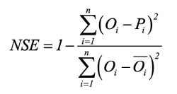 (9)
(9)
where Oiand Pi are the observed and predicted flow at time t, respectively; is the mean observed flow; and n is the number of observations.
Study area and data
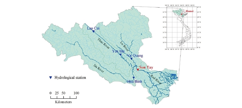
The study area is the basin of the Red River system, one of the largest river basins in Vietnam. The data collected for this study were the average daily discharges observed at five hydrological stations. The four-gauge stations located in the upstream region are the Lao Cai and Yen Bai stations on the Thao River, Hoa Binh station on the Da River, Vu Quang station on the Lo River, and the target station, Son Tay, located on the Red River. The locations of the gauge stations in the study area are shown in Fig. 3.
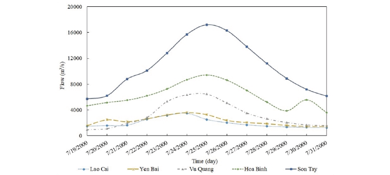
The Red River system is a combination of three major river branches, namely Da River, Thao River and Lo River, in which Thao River is considered as the mainstream. The flow on the Da River accounts for about 47% of the total water volume of the Red River, followed by Lo River and Thao River with the respective rates of 28% and 25%. In addition, the flow on the Red River has a large fluctuation range due to the annual water level changes range from 5 m to 8 m. In particular, this fluctuation level can reach 14 m for the years with large floods. The rainy season usually starts from the end of April to November, the flow during this period accounts for about 70 - 80% of the total water volume of the year. Moreover, flooding on the Red River is often a combination of flood flow of two or three main tributaries. The flood peaks on these branches have different peak values as well as peak appearance time. Fig. 4 illustrates a typical flood in the year of 2000 and the observed flowrates at the hydrological stations.
The target hydrological station is located in Son Tay district, northwest of Hanoi, and its position plays a vital role for the city, which is the cultural and political center of Vietnam. The findings of this study will serve as a precursor to developing an early flood warning system on the Red River for Hanoi city. The input data for this study were a time series of daily flow data recorded at the hydrological stations for 15 years from 1972 to 1978 and 1997 to 2004. In our research, the flowrate was measured in cubic meters per second (m3/s).
The dataset of the average daily discharge measured at the five hydrological stations was divided into three sections, including two main sections and one sub-section, for different purposes. The first section was a series of measured actual flow data over 14 years (from 1972 to 1978 and 1997 to 2003), which was used for the training phase and model evaluation. The second section was a set of observed discharge data from January 1 to December 23, 2004, and was used to test and select the best set of parameters for the LSTM model. The final section was a small dataset collected from December 24 to 31, 2004, and was used as an unseen dataset to assess the performance of the model with three specific prediction cases, i.e., one-, two-, and three-day forecasts, at Son Tay hydrological station.
Model design
The LSTM network model developed in this study depends on open source software, and Python (Rossum, 1995) is the dominant programming language throughout the research. Furthermore, we selected TensorFlow as the framework for this study, which was developed by Google for machine learning and deep learning purposes and applications. In addition, libraries, such as Numpy (Van Der Walt et al., 2011) and Pandas (McKinney, 2010), were imported to support data processing and management.
Unlike conventional hydrodynamic models, these models must resolve complex Saint-Venant equations, which combine the mass and momentum conservation equations. In contrast, DNN models learn these physical principles in the training process from input data and evaluate the performance through the verification process and produce streamflow forecasts that are as accurate as possible. Several parameters and the structure of the LSTM model are suggested to ensure that the model can perform as best as possible after the training and testing phases. The details of the suggested parameters for the model are presented in Table 1.
The input data of the model were the observed daily flowrates measured at the five hydrological stations in the study area. However, there have been some minor modifications to the format of the input data for the model.
This change allows the model to learn more efficiently and make better predictions. At any time, the input data are formatted into sequential data, rather than just the individual data points. The selected sequence length for the model is a series of five days. That is, the flow data from the five most recent days will be adopted as input data to the LSTM model. The data sequence length is the five most recent days corresponding to the five most recent measured time steps. For the proposed LSTM model, sequence length is one of the key factors that significantly affect model performance. However, there is no specific reference for selecting this parameter. Moreover, this value typically depends closely on data characteristics and observation frequency. For example, the data observed daily will be different from the observed data hourly. In addition, if the sequence length is small (1 or 2), the model can save considerable computational time, but sometimes the performance is not as expected. Meanwhile, increasing this value will make the model complicated and consume a large amount of computing resources during the training process. This may cause the model faces to similar problems in the RNN models. Another important point is that the model performance has not changed significantly when increasing the sequence length to 10. Therefore, the sequence length of 5 is recommended for this paper.
Training parameters, such as the number of units or number of epochs, were selected as shown in Table 1. The number of units is the number of LSTM units in a layer at every time step of the network. Different numbers of units in the LSTM model are selected to evaluate the importance of the number of units when building a prediction model. Furthermore, one epoch can be defined when an entire dataset is passed forward and backward through the neural network once. The performance of the predictive model is recorded after each training and testing (one epoch) step. In this study, the maximum number of epochs of 100,000 were selected to ensure that the predictive model could record all the necessary information. Several other techniques, such as the dropout technique to prevent overfitting (Srivastava et al., 2014) or optimization algorithm for error optimization in the loss function, is applied to improve the efficiency of the model. The Adam optimization algorithm was selected in this study (Kingma and Ba, 2014).
Results and Discussion
Testing results
The predictive models were validated using data not used for training (the second dataset) and evaluated using the NSE and RMSE metrics when comparing the observed and predicted data. With the parameters and structure selected above, the LSTM model was applied to perform one-, two-, and three-day discharge forecasts at Son Tay gauge station.
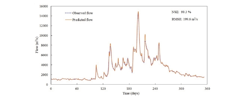
When predicting one day ahead, the best results of the testing phase corresponding to the different cases are summarized in Table 2 and detailed in Fig. 5 and 6.
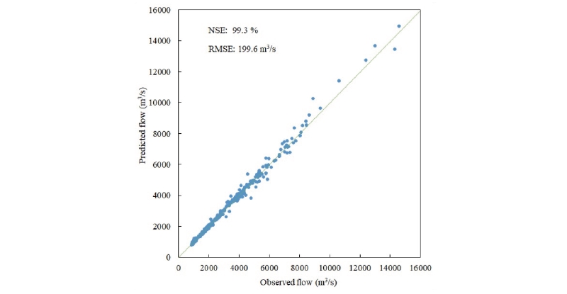
The result of the one-day flow forecast model in Table 2 indicates that the proposed DNN model made predictions with high accuracy. The NSE value reached 0.992, and the mean RMSE was approximately 202 m3/s for all three cases. The predictive accuracy in all cases was highly stable and was almost maintained when the number of units in the LSTM cell changed. Fig. 5 and 6 demonstrate the close correlation between the predicted and observed data of case 1, which was the one-day flow forecasting model. The equivalent RMSE value was just 199.6 m3/s.
|
Table 2. Summary of the best results for one-day flow forecasting. 
|
|
RMSE, root mean square error; NSE, Nash-Sutcliffe Efficiency. |
The flood peak was predicted to occur at the same time as the observed flood peak at Son Tay hydrological station on July 24. The absolute error value in the flood peak forecast was only 339 m3/s, and the observed peak value was 14,600 m3/s. The relative error in this case was approximately 2.3% and the forecasted flood peak was higher than the measured peak.
According to the results in Table 2, when the number of units increased, the number of computations required to minimize the loss function decreased (i.e., the epoch decreases). Increasing the number of units in an LSTM cell would increase the complexity of the model, and more time would be required to calculate and update all weights per epoch. However, the results illustrate that the convergence rate of the model is also proportional to its complexity. If there were 20 LSTM units per cell, the model underwent 3,200 iterations to attain the minimum RMSE value, instead of the 22,900 iterations when there were 5 units.
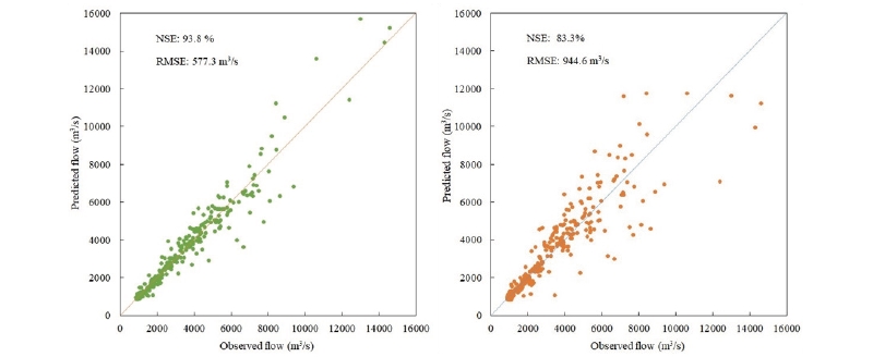
For the two- and three-day flow predictions, the best predictive results of the different cases are summarized in Table 3 and Fig. 7.
|
Table 3.Summary of the best results for the two- and three-day flow forecasting models. 
|
|
RMSE, root mean square error; NSE, Nash-Sutcliffe Efficiency. |
For the two- and three-day predicted flows, predictive modeling produced the best results when there were 10 units or LSTM units. The NSE values for these two cases were approximately 0.938 and 0.833, respectively. For each forecasting model, the difference in accuracy was insignificant, although the number of units varied from 5 to 20. The differences in the NSE value were only approximately 0.43% and 0.79% for the two- and three-day prediction models, respectively. The best performance of the two-day prediction model was achieved after 5,200 iterations (each iteration is equivalent to one epoch). In this case, the minimum loss function value was equivalent to an RMSE of 577 m3/s. In contrast to the two-day prediction model, the three-day flow forecast model only took 2,200 iterations to optimize the loss function. Optimal performance was achieved when the RMSE value was almost 945 m3/s.
Fig. 6 and 7 indicate the correlation between the predicted and observed values when these data pairs are represented in the three best cases of the flow forecast models at Son Tay station. Each pair of data is represented by a blue dot on the figure. The closer these points are to the diagonal of 45 degrees, the better the predictive model. It can be seen that, when forecasting further into the future, the predictability of the model declined. The accuracy of the three-day prediction model was 0.833, while that of the one-day prediction model was 0.993, and that of the two-day flow prediction model was 0.938.
The results in Table 3 illustrate a similar development in the two- and three-day flow forecast models. As the number of units per cell increased, the predicted model reached the minimum RMSE value more rapidly (i.e., the number of iterations or epochs reduced). While the number of units in the two-day forecast model increased from 5 to 20, the number of iterations required for the model to reach the optimized value decreased from 6,100 to 1,600. Meanwhile, the three-day forecasting model exhibited faster convergence rates, i.e., the number of epochs decreased from 4,900 to 1,100 with the same change in the number of units as discussed above.
In addition, the author developed several different scenarios to evaluate the performance of the proposed model. The sizes of the training and test datasets were further redistributed in a manner that decreases the size of the training dataset and increases the size of the test dataset. The purpose of this was to evaluate the quality and size of the data for the training process. The results show that, with the current data division, the models are more stable and efficient than others. However, the change is slight, with the accuracy fluctuating by approximately 1 - 2% (depending on the predicted case) from that selected above.
Forecasting results
After training and testing, the best set of parameters of the model corresponding to the predicted cases was selected (Table 2 and 3). The third dataset is a sequence of eight days of measured flow data from December 24 to 31, 2004. The data for the first five days were used as input data for the model to produce forecasts for one, two, and three days in the future. The data for the following three days were used to compare the flowrate between the predicted and measured values in each forecasted case and evaluate the effectiveness of the LSTM model. This is an independent dataset that has not been used previously. The model took five-day observation data from December 24 to 28 to produce one-, two-, and three-day flow forecasts (corresponding forecasts for the 29, 30, and 31 of December). The results of the DNN model are presented in Table 4.
From the forecasted results presented in Table 4, it can be seen the absolute error in the case of forecasting the flow for one day was only 11.0 m3/s, as the observed value was 1,430 m3/s on December 29. The value of this absolute error indicates the accuracy of the model, which exceeded 99% in this case. In addition, the accuracy of the three-day flowrate forecast was approximately 82% (the observed value recorded on December 31 was 1,670 m3/s). These results confirm that the proposed LSTM model performed well and the predicted results were reasonably stable.
Conclusions
In this study, the authors constructed a DNN model based on an ANN model to predict one-, two-, and three-day flows at Son Tay station on the Red River. The LSTM model takes a series of discharge data measured at five hydrological stations as the input data without requiring rainfall data, water levels, as well as topographic characteristics. The parameters established in the model were selected and carefully assessed through training, testing, and the use of algorithms to optimize the errors in these processes. The results of the testing process indicate a close correlation between the predicted and observed values. The accuracy of the model decreased when the forecasting time step increased.
The aforementioned results indicate the outstanding performance of the LSTM model for forecasting the flowrate at Son Tay station for one, two, and three days in advance. In addition, this model is data-driven and is more simple than other sophisticated hydrodynamic models as it does not require many types of data. As a result of this study, the proposed model can be used to construct a real-time flood warning system on the Red River and other river basins in Vietnam.


