Introduction
Wind erosion which can degrade soil, air, and water resources is a serious problem on agricultural lands throughout Korea as well as the world. Initiation of soil erosion by wind occurs when the wind speed exceeds the saltation threshold speed for a given soil (Skidmore and Tatarko, 1991). After initiation, the duration and severity of an erosion event is determined by the wind speed distribution and the evolution of the surface condition (Wagner et al., 1992; Tatarko and Wagner, 2007). Researches about wind erosion have shown that removal of the most fertile parts of the soil including clays and organic matter by wind erosion lowers soil productivity (Lyles and Woodruff, 1960; Armbrust, 1984; Lyles and Tatarko, 1988; Blanco-Canqui and Lal, 2009). Therefore, accurate prediction of soil loss by wind is essential for conservation planning, natural resource inventories, and reducing air pollution caused by wind erosion.
Wind erosion models can be used for a variety of purposes such as estimation of the on-site and off-site consequences of wind erosion and development of erosion control measures. The Wind Erosion Equation (WEQ) developed more than forty years ago was the most widely used method to assess soil loss by wind from agricultural fields (Woodruff and Siddoway, 1965; Fryrear et al., 1991; Fryrear et al., 1998a; Zobeck et al., 2001; Panebianco and Buschiazzo, 2008). However, the application of WEQ required a number of efforts to improve the accuracy, ease of application, and range of WEQ (Fryrear et al., 1998a; Fryrear et al., 2000; Tatarko et al., 2013). Most of the current models which were derived from the initial researches on wind processes and dynamics of wind erosion models conducted by Chepil (1945a, 1945b, 1945c) can estimate the rate of soil erosion from small-scale to larger geographic areas on a regional and national basis (Hagen et al., 1995a, Hagen et al., 1995b; Borrelli et al., 2015; Borrelli et al., 2016).
WEPS developed by the USDA-Agricultural Research Service was intended to improve technology for assessing soil loss by wind from agricultural fields and to provide new capabilities, assessing plant damage, calculating suspension loss, and estimating PM-10 emissions from the field. It might replace the predominately empirical WEQ as a prediction tool for those who assessed offsite impacts from to wind erosion (Hagen, 1995; Tatarko, 1995; Tatarko et al., 1995; Wagner and Ding, 1995; Wagner, 1996; Zobeck and van Pelt, 2006). It also provided the user with spatial information regarding soil flux, deposition, and loss from specific regions of a field over time (Retta and Armbrust, 1995; Wagner and Hagen, 2001). Unlike WEQ (and RWEQ), WEPS in which the erosion submodel is one of 7 major submodels is a process-based, daily time-step model that simulates weather, field conditions, and erosion under a wide range of conditions in the U.S. and easily adapted to other parts of the world (Retta and Armbrust, 1995; Steiner et al., 1995; Wagner, 1996; Funk et al, 2003). WEPS can simulate complex field shapes, barriers not on the field boundaries, and complex topographies. The simulation to estimate soil loss by WEPS depends much more on the relationship among erosion events, than on a good agreement for one single event (Funk et al., 2003). WEPS requires wind speed and direction to simulate the process of soil erosion by wind. These and other weather variables are needed to derive temporal changes in hydrology, soil erodibility, crop growth, and residue decomposition in WEPS (Wagner, 2011).
Due to lack of variable data needed for simulation in Korea, there is few published researchs testing WEPS to estimate soil loss based on single erosion events and outputs from the erosion submodel under arable conditions. Soil loss predicted by WEPS like other previous models is expressed as mass per area, that can’t reflect the actual changes of soil physical properties. Therefore, it may be difficult to develop the adequate control method to prevent soil in arable land. The objective of this study is to compare and verify the applicability of the WEPS for prediction of soil loss by wind and we were measured as mass per area in arable land using available databases by WEPS and calculated soil loss as depth converted data of WEPS under same conditions.
Concepts and application of WEPS
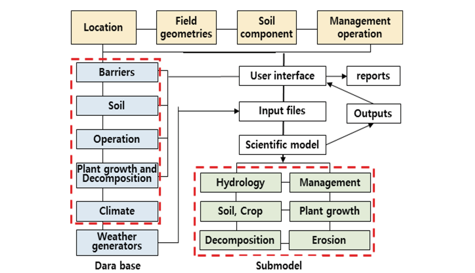
WEQ predicts only long-term, average soil loss for a single, uniform, isolated field in which erosion occurs along line-transects (Woodruff and Siddoway, 1965). In contrast, WEPS provides capability to handle nonuniform areas inside the simulation region to obtain predictions for specific areas of interest (Hagen et al., 1999). The structure of WEPS as a continuous, daily, time-step model is modular and consists of database and 7 submodels under 4 main factors consisted of location, field geometries, soil component, and management operation, covering at least a single year (Ankeny et al., 1995; Durar and Skidmore, 1995; Hagen, 1995, Seo et al., 2020). Each individual submodel controls the sequence of calculations within itself. Submodels in WEPS simulate the general processes that control both the surface temporal properties and the erosion processes, using parameters obtained from the databases for specific soil, crop, and management actions (Hagen et al., 1996; Hagen et al., 1999). Most of the submodels within WEPS use daily weather as the natural driving force for the physical processes that change field conditions. The hydrology submodel accounts for changes in the temperature and water status of the soil. Changes in the soil properties among management events are simulated in the SOIL submodel (Hagen et al., 1996).
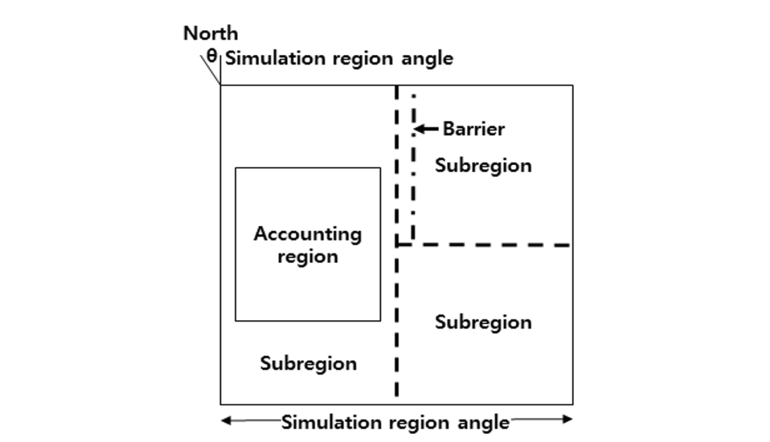
For a WEPS simulation to predict soil loss in a field, the erosion submodel uses some parameters supplied by other submodels that describe the soil surface, flat biomass cover, standing biomass leaf and stem areas, and weather to decide if wind erosion can occur in a simulation region. The erosion submodel considers the simulation region to be rectangular and composed of one or more rectangular fields with differing surface conditions, and the settled bulk density in any layer of soil will be estimated at less than a 30 cm in depth. The erosion process is simulated as the time-dependent mass conservation using linked partial differential equations for three size classes of eroding soil (Hagen, 1995). The geometry of the simulation region including any subregions should be specified along with input initial conditions for the surface and 4 to ten layers (Fig. 1). These are saltation and creep size (0.1 to 2.0 mm), suspension size (< 0.1 mm), and PM-10 size (< 0.01 mm). However, the erosion submodel is not called unless maximum daily wind speed at 10 m height reaches 8 m·s-1 (Tatarko et al., 1995). One problem may occur if a daily erosion event causes large gradients of variables to develop across a single subregion. This gradient may affect the erosion on subsequent days for each subregion to begin the daily erosion (Hagen et al., 1996). The output of WEPS indicates average soil loss/deposition over selected time intervals and accounting regions within the simulation region which is a field or a few adjacent fields (Fig. 2). Multiple and overlapping accounting regions can be selected to obtain averaged output over various spatial scales in the simulation region (Wagner, 1996).
Simulation by WEPS requires wind speed and direction to reflect the process of soil erosion by wind. Weather variables are needed to drive temporal changes in hydrology, soil erodibility, crop growth, and residue decomposition. Surface properties, such as crust generation, coverage fraction, random and oriented roughness, density, stability and thickness, and loose erodible material on surfaces can be accounted for in the soil submodel (Wagner and Ding, 1995). The erosion submodel performs the following calculation functions: 1) friction velocities on the roughness of the surface, 2) static threshold friction velocities, 3) soil loss/deposition at each grid point (Wagner, 2011). To carry out these functions, the erosion submodel requires parameters supplied by other submodels describing the soil surface, flat biomass cover, standing biomass leaf and stem areas, and weather in a simulation region. Then, the submodel simulates the process of soil movement if erosion can occur (Hagen, 1995).
Comparison and validation of WEPS erosion submodel
It is imperative to validate the performance of erosion submodel on arable land because wind erosion models are used for various purposes to predict soil loss by wind at the on-site and off-site fields. In this investigation to compare and validate the results between the predicted by WEPS and soil depth converted from the predicted, we selected the experimental results based on single erosion events and outputs from the erosion submodel of WEPS published by Hagen in 2004. The individual experimental sites were a 2.5 ha circular areas that were tilled and located within larger fields that remained in relatively nonerodible condition, permitting collection of erosion data regardless of wind direction. The selected fields in that experiment included a wide range of soils with sand fractions ranging from 29% to 90% with relatively low calcium carbonate content (Table 1).
To figure out soil loss predicted by WEPS, they fitted the measured point-discharge cluster data to empirical equations to estimate soil discharge at 180 m downwind from the nonerodible boundary. The discharge for each storm then was divided by 180 to provide an estimate of soil loss per unit area for a 180 m long, 1-m wide, strip of field (Hagen, 2004).
To compare and validate the soil loss predicted by WEPS whether the results represented the actual changes of soil physical properties as soil depth, we converted soil loss expressed as mass per area into depth based on bulk densities of top soil layer as follows;
 (1)
(1)
Whereas, designated depth of soil could be determined as the depth to be investigated and mass and area of soil loss expressed as pound (l b) in WEPS were converted into kg and 10 a by multiplying 0.4534 and 0.247 as follows, respectively.
Mass of soil (M·10 a-1) = area (acre) × 0.247 × depth (L) × bulk density (BD, M·L-3) (2)
Bulk density (BD) = mass of dry soil (M)/volume of soil (L3) (3)
Mass of soil (M, kg) = mass (l b) × 0.454 (4)
Area (10 a-1) = area (acre) × 0.247 (5)
Generally, the BDs of top 20 cm in the cultivated arable land ranged from 1.1 g·cm-3 to 1.3 cm-3 regardless of soil texture and organic matter content due to mechanical manipulation to improve soil physical properties. Table 2 shows the calculated soil depth based on the observed and predicted soil loss expressed as mass per area. The soil loss calculated as soil depth for single event was decreased with increasing BD and maximum soil depths for 60l b soil loss reached from 2.08 cm to 2.47 cm as the BD changed from 1.3 ton·m-3 to 1.1 ton·m-3. For this, the soil loss obtained by single erosion events from the erosion submodel of WEPS may not reflect soil loss for multiple erosion event.
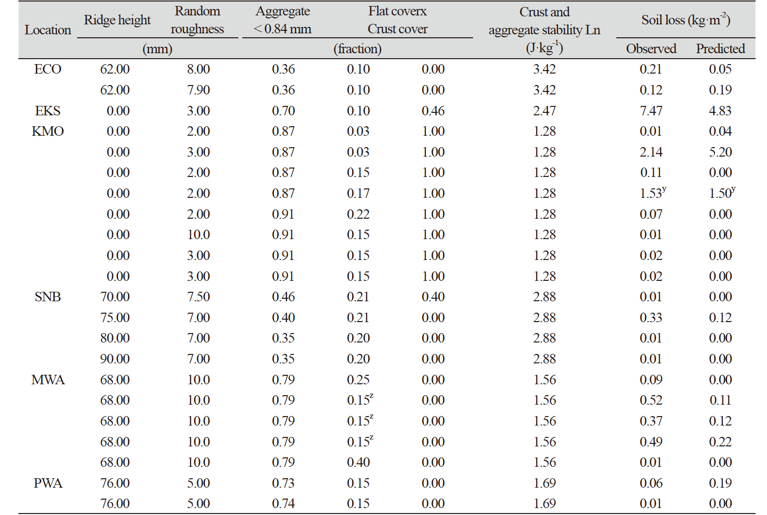
Table 3 shows the field surface conditions without the field surface parameters in the storm simulations used in Hagen’s results. They assumed that the air dried conditions of surface soil during the erosion events occurred when test site conditions were not uniform and had small inclusions with higher erodibility than the average conditions in the model inputs. Aggregate and crust dry stabilities were assigned average values based on soil texture. In several events, the soil loss predicted by model estimated zero erosion when measured amounts of soil loss were less than 0.1 kg·m-2. But he concluded that this should be of little consequences for practical model applications (Hagen, 2004).
Data analyses procedures for the horizontal soil flux trapped by the catchers in each cluster was fitted to a 4-parameter equation as suggested by Vories and Fryrear (1991).
f(z) = azb + c·exp(dz) (6)
Where f (z) is horizontal flux (kg·m-2) per storm at height z (m), and a, b, c, d’s are fitting coefficients. The vertical profile of the horizontal flux as shown in Eq. (6) was then integrated to a height of 2 m to determine the soil discharge (kg·m-1) passing each cluster location. Calculation of wind direction and upwind distance to the edge of the field were completed for each cluster.
The empirical equation providing the best fit to most of the cluster discharge data was of the form shown in Eq. (6) below;
q = f + gXn (7)
Where q is downwind horizontal discharge (kg·m-1), X is downwind distance from nonerodible boundary, and f, g, h are empirical fitting coefficients.
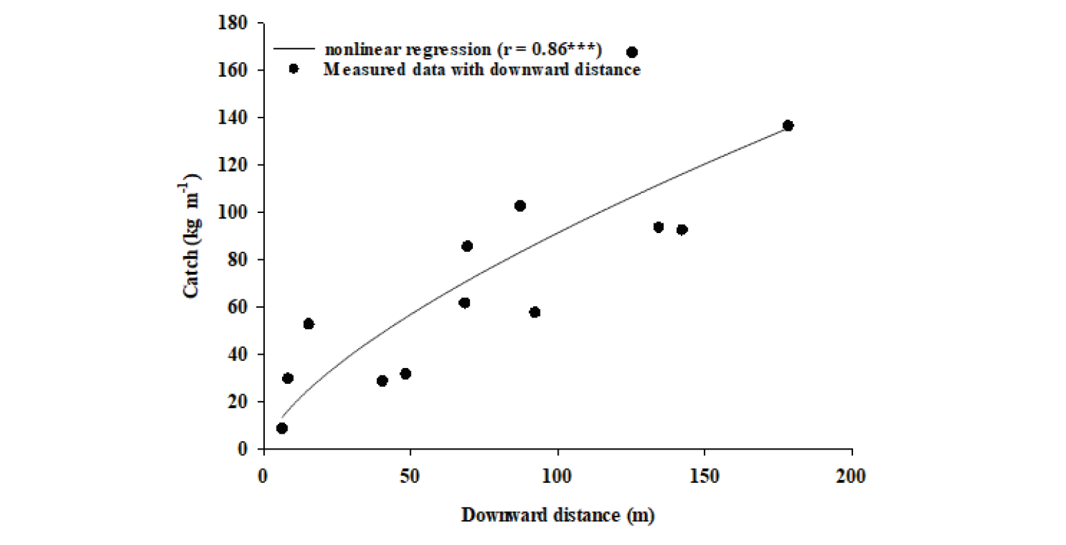
To validate the Eq. (7), Hagen (2004) selected data from a 1997 storm at Big Spring (BSTX). In this, the wind statistics included the maximum and average wind speed, and a wind factor related to erosive wind energy for each daily storm that assumed a threshold wind speed of 5 m·s-1 at a 2 m height as of Fryrear et al. (1998b). Also, three parameters for a Weibull cumulative wind speed distribution of the form were used to estimate wind speeds during each storm day. Eq. (7) showed a relatively good fit (r = 0.86***), while the shape of the downwind discharge curves varied between convex depending upon field surface conditions, as shown in Fig. 3.
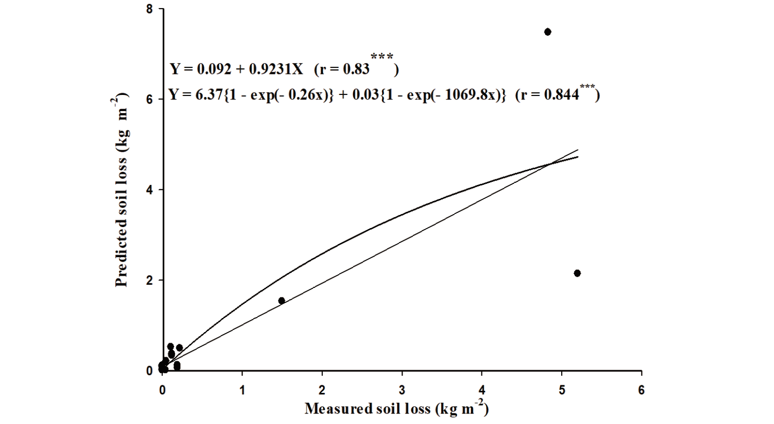
Analysis of the storm data was compared with linear regression and nonlinear regression using a power equation with the form of Eq. (2). The results of the average storm loss from the cluster measurements extrapolated using Eq. (2) to 180 m downwind showed reasonable agreement between predicted and observed erosion (r = 0.83*** as linear and 0.84*** as nonlinear regression) with a slope less than one and an intercept greater than zero (p = 0.05 for both analysis) (Fig. 4). The results analyzed by linear regression showed that the predictions were close to the 1 : 1 line if storm losses were less than 1.75 kg·m-2 although the intercept calculated by regression equation was slightly less than zero. But predicted soil loss by WEPS erosion submodel deviated from the regression line if the measured soil loss values were greater than 0.25. From these two prediction of soil loss calculated by soil erosion submodel, it can be only effective in a limited range under given soil and climatic conditions.
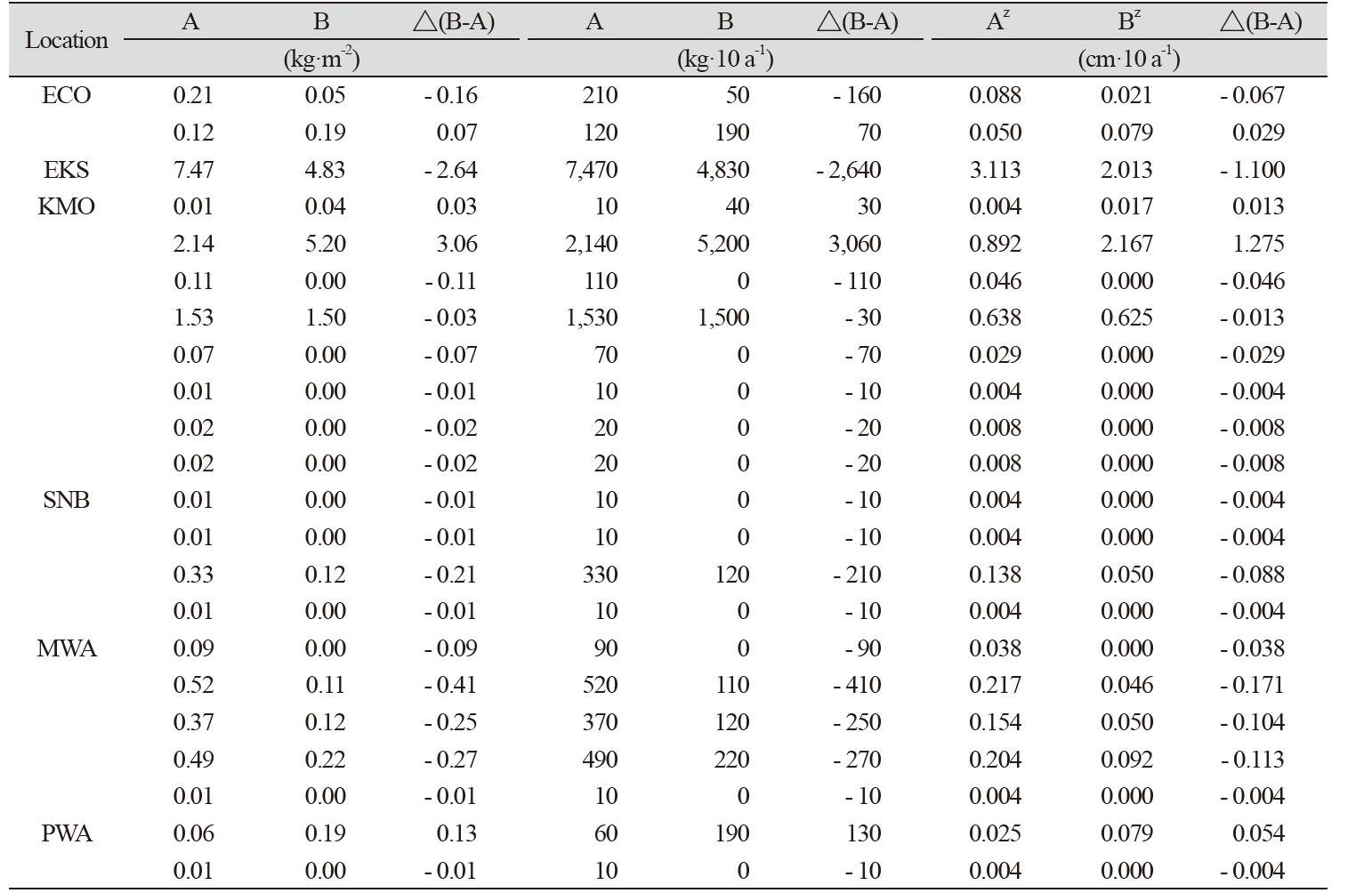
To predict the soil loss using soil erosion submodel, it needs many soil factors as well as parameters related to daily storm including maximum and average wind speed. However, the values about soil loss between observed and predicted did not show any relationship as shown in Table 4. For example, the soil losses for two storm events about ECO of which soil texture was clay loam showed opposite values although the field conditions for selected erosion events were almost same as seen in Table 4. In several other cases, the model estimated zero erosion while there were soil loss for the observed ones. This could be caused by test site conditions of which sites are not uniform and higher erodibility causes smaller inclusions than the average conditions that are assumed in the model inputs as seen in the values for Knuth-Morris-Pratt (KMP) that showed no soil loss for predicted values. The maximum differences between observed and predicted loss occurred during large erosion events where the predicted values were frequently less than those observed (Fig. 4). For this, Hagen (2004) concluded that there are two probable causes for the under- and over-prediction of soil loss for the observed ones. First, model requires more inputs to configure soil loss, so average parameter values for the specific soils were substituted for these inputs. Second, weathering and prior erosion may have increased the soil erodibility after the time of the reported surface measurements (Hagen, 2004). Probably, it is likely that the soil conditions were more erodible than reflected in the input surface conditions when erosion occurred in the field. But these explanations are not good enough to account for these problems.
Calculations of soil loss by WEPS implying erosion submodel for single event were a daily time step model that simulates weather and field conditions (Hagen et al., 1995). Soil loss was represented by soil loss per square meter in soil erosion investigation, even in erosion model. But this couldn’t represent how much soil was lost in depth from the field. The soil loss per square meter was interpreted as the depth of soil per 10 a-1 by assuming soil bulk density of 1.20 tons per cubic meter (Table 4). Depth of soil lost by wind ranged from 0.004 to 3.113 cm and from 0 to 2.013 cm·10 a-1 for observed and predicted, respectively. For the depth of soil of observed and predicted ones lost by wind, we need to verify whether it may represent the actual soil depth for single event although the model provided reasonable estimates (r = 0.84***) of soil loss.
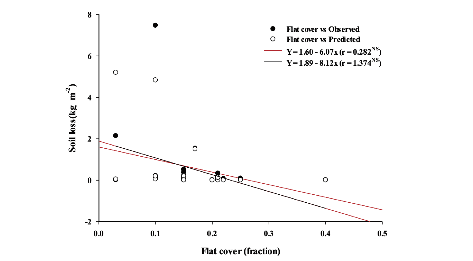
The threshold of soil loss in the erosion model was calculated based on surface conditions of: random and oriented roughness; flat cover, crust, and rock cover; cover of loose, erodible aggregates on the crust; aggregate size distribution and density of uncrusted surface; and surface wetness (Funk et al., 2003). With these factors, we could figure out correlation to prove reliability for the result of soil loss. Fig. 5 shows the soil loss for flat cover for individual storms with linear regression analysis based on the result of Hagen (2004). As seen in figure, linear regression were weakly correlated with flat cover in all the average storm loss from the cluster measurements in a linear way. This indicates that flat cover has a low effect on wind erosion on the average storm loss from the cluster measurements. Considering for individual storms with linear regression analysis, we may have to apply proper parameters with respect to all available information, in order to reduce the uncertainty and to minimize subjectivity.
Conclusion
The output of WEPS for single erosion event indicates average soil loss/deposition over selected time intervals and accounting regions within the simulation region in a field or a few adjacent fields. For evaluation based on the data by Hagen (2004), the model tended to follow the 1 : 1 line between predicted and measured value for soil losses only less than 2 kg·m-2 whereas the differences between observed and predicted loss occurred during erosion events when the predicted values were less than those observed ones because the initial field surfaces were not always uniform as assumed in the model although the model provided reasonable estimates (r = 0.84***) of soil loss. As partial account for these problems, the changes in surface conditions were simulated on a daily basis in the completed WEPS model. The model estimated zero erosion when small amounts of erosion occurred. It can assume that the field conditions were more erodible than reflected in the input parameters in the field. Thus, the correlation between the values about soil loss between observed and predicted was not significantly different, and that between flat cover in storm loss form the cluster and soil loss, respectively, resulting in reduction of the uncertainty and minimization of subjectivity. Therefore, these explanations are not good enough to account for these problems. As calculated soil depth by wind, the ranges of predicted and observed values were 0 - 2.013 cm·10 a-1 and 0.004 - 3.113 cm·10 a-1, respectively. It may also be too high for given wind condition of single storm event. Conclusively, WEPS to predict soil loss for given soil condition requires more site-specific parameter although this should be of little consequence for practical model applications. Therefore, we need to develop the parameters to apply WEPS to predict soil loss by wind in Korea.
Acknowledgements
This subject is supported by Korean Ministry of Environment as “The SS (Surface Soil conservation and management) projects;2019002820004”
Authors Information
Kyo-Suk Lee, https://orcid.org/0000-0002-8668-5500
Il-Hwan Seo, https://orcid.org/0000-0003-0527-5938
Sang-Phill Lee, Department Kangwon Institute of Inclusive Technology, Kangwon National University, Research Professor
Chul-Soon Lim, https://orcid.org/0000-0003-2271-2204
Dong-Sung Lee, https://orcid.org/0000-0003-2234-6996
Se-Won Min, Department of Bio-environmental Chemistry, Chungnam National University, Undergraduate student
Hyun-Gyu Jung, Department of Bio-environmental Chemistry, Chungnam National University, Adjunct Professor
Jae-Eui Yang, Department of Biological environment, Kangwon National University, Professor
Doug-Young Chung, https://orcid.org/0000-0001-7948-1297


